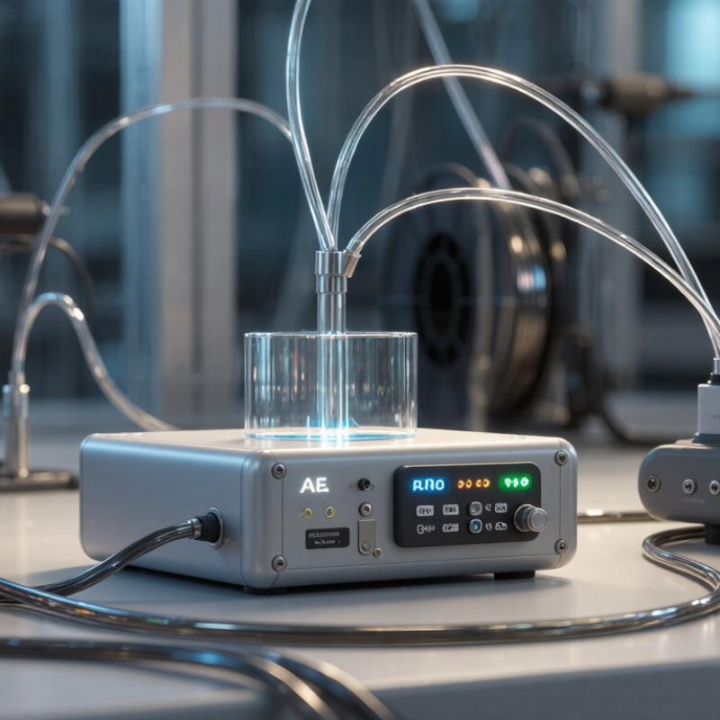
A 1528–1603 nm ASE source does not sit entirely inside the conventional C- and L-band definitions. The commonly used C-band span is about 1530–1565 nm; L-band extends roughly from 1565 to 1625 nm. So this source begins just below the usual C-band edge, crosses the C/L boundary, and ends within L-band. The edge matters. A test setup labeled “C+L” may still need to account for output near 1528 nm.

In frequency terms, 1528–1603 nm is approximately 196.2–187.0 THz. ITU-T G.694.1 defines DWDM frequency-grid spacing, including 100 GHz spacing; near 1550 nm, that is about 0.8 nm between channels. This is useful context, not a guarantee that an ASE spectrum will be flat or channel-aligned. Check the measured spectrum, power density, and ripple across the full wavelength span, especially around 1565 nm. A small mismatch can be easy to miss. The band boundary itself is a convention, and I would verify the supplier’s stated measurement limits rather than assume every instrument uses the same cutoff.

For a 1528–1603 nm ASE source, spectral flatness should be judged across the entire 75 nm span, not from a smooth-looking center section. Edge behavior matters. A spectrum that appears even near 1565 nm may still roll off near either endpoint. Compare the maximum and minimum power spectral density across the specified band, and note the measurement resolution and test conditions. A plot without these details is hard to evaluate.

Match the flatness requirement to the application’s usable wavelength range; a tighter specification is not automatically better if only part of the band is needed. Ask for measured data across 1528–1603 nm, including stated limits and test conditions. If possible, inspect raw traces rather than relying only on a single flatness figure. I would not assume a perfectly level spectrum, either; real measurements include uncertainty, and that deserves a note.

An ASE source covering 1528–1603 nm should be chosen for the receiver’s usable band, not its headline output alone. Build the link budget from launch power, then subtract fiber, connector, splice, filter, and receiver losses. ITU-T Recommendation G.652 gives a maximum attenuation coefficient of 0.30 dB/km at 1550 nm for specified single-mode fiber. On a 20 km path, that can mean 6 dB of fiber loss before connectors. Small losses add up. Leave margin for temperature changes, aging, and repairs.

For a 1528–1603 nm ASE source, treat 50 GHz as a measurement reference, not a discrete-channel guarantee. At 1550 nm, 50 GHz corresponds to about 0.40 nm in wavelength. The equivalent interval changes across the band: it is slightly narrower near 1528 nm and wider near 1603 nm. Small detail, real consequence.

Tip: Compare usable spectral power across the full range, then check the spectrum with resolution fine enough to distinguish features about 0.40 nm apart near 1550 nm. A coarse analyzer can blur ripple into an apparently smooth trace. Confirm whether the stated bandwidth means a 3 dB width, a flatness range, or merely detectable output. These are not interchangeable.

Tip: Ask for power density, ripple, and stability data under stated operating conditions. If your setup uses 50 GHz filters, verify passband alignment and guard margins rather than matching numbers on paper. Real filters have edges, and connectors add loss. A single scan can mislead, so repeat it after warm-up and record the settings. It takes extra time, but the check is worthwhile.